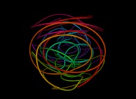
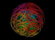
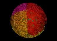
Space filling Curves and Beyond:
From Squares and Cubes to Surfaces (bidimensional Manifolds) and tridimensional Manifolds
CMAP (Centre de Mathématiques APpliquées) UMR CNRS 7641, École polytechnique, Institut Polytechnique de Paris, CNRS, France
[Site Map, Help and Search [Plan du Site, Aide et Recherche]]
[The Y2K Bug [Le bug de l'an 2000]]
[Real Numbers don't exist in Computers and Floating Point Computations aren't safe. [Les Nombres Réels n'existent pas dans les Ordinateurs et les Calculs Flottants ne sont pas sûrs.]]
[Please, visit A Virtual Machine for Exploring Space-Time and Beyond, the place where you can find more than 10.000 pictures and animations between Art and Science]
(CMAP28 WWW site: this page was created on 04/17/2023 and last updated on 01/24/2025 18:15:23 -CET-)
[en français/in french]
Contents:
1-Georg Cantor:
In the second half of the nineteenth century, Georg Cantor was one of the founders of set theory
by questioning the concept of infinity. Using the notion of the power set (ie. the set of all subsets of a given set),
he showed that there was not one infinity, but an infinity of infinities.
The smallest infinity is that of the integers N: the countable infinity.
The notion of bijection between two sets is then fundamental: two sets have the same cardinality ("are the same size")
if there exists a bijection between them.
It is almost paradoxical that sets such as the even numbers, the rationals, the algebraic numbers, etc.
are in bijection with N and are therefore countable.
However, using a proof by contradiction of astonishing simplicity,
Cantor showed that this was not the case with the set of real numbers R:
R is not countable.
Note that knowing whether there are sets of intermediate size between N and R is (unfortunately...) an
undecidable (the so-called Continuum Hypothesis)
of ZFC (Zermelo, Fraenkel and axiom of Choice) set theory.
Beyond R, there are therefore an infinity of increasingly enormous sets obtained,
for example, by iterating the definition P of the power set: {E,P(E),P(P(E)),...}.
But despite this, Georg Cantor showed that R, R2,... Rn,... had the same cardinality.
2-David Hilbert, Giuseppe Peano and more:
Building on this result, David Hilbert, Giuseppe Peano,
and others imagined curves (parameterized in R) filling a square (in R2).
One simple way to proceed is to start with a so-called generating curve  that will be reduced
and transformed by repeating the process an infinite number of times.
To illustrate this process, here is a specific generating curve
  and the four transformations
  it must undergo at each iteration.
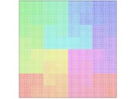
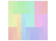
Here are the five first bidimensional Hilbert curves with an increasing number of iterations
:


See the construction of some of them
:


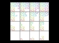
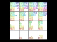

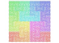
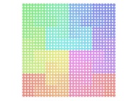
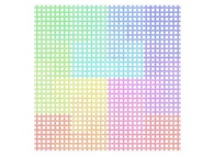
Here are some examples of Hilbert-like bidimensional curves using different generating curves
:




This process can be generalized, and it is thus possible to fill a cube (in R3)
using curves (still parameterized in R). Here is one of the generating curves  ,
and again, a specific generating curve
  allows us to understand
the eight transformations
  it undergoes at each iteration.
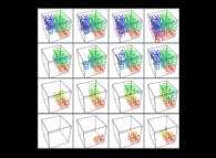
Here are the four first tridimensional Hilbert curves with an increasing number of iterations
:


See the construction of one of them
:


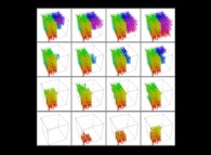
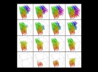
Here are some examples of Hilbert-like tridimensional curves using different generating curves and in
particular "open" knots
:


3-Tridimensional Surfaces (Bidimensional Manifolds):
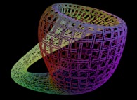
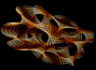
Many surfaces -bidimensional manifolds- in a tridimensional space
can be defined using a set of three equations:
X = Fx(u,v)
Y = Fy(u,v)
Z = Fz(u,v)
with:
u ∈ [Umin,Umax]
v ∈ [Vmin,Vmax]
For example:
Fx(u,v) = R.sin(u).cos(v)
Fy(u,v) = R.sin(u).sin(v)
Fz(u,v) = R.cos(u)
with:
u ∈ [0,pi]
v ∈ [0,2.pi]
defines a sphere with R as the radius and the origin of the coordinates as the center.
[Umin,Umax]*[Vmin,Vmax] then defined a bidimensional rectangular domain D.
                       v ^
                         |
                    V    |...... ---------------------------
                     max |      |+++++++++++++++++++++++++++|
                         |      |+++++++++++++++++++++++++++|
                         |      |+++++++++++++++++++++++++++|
                         |      |+++++++++++++++++++++++++++|
                         |      |+++++++++++++++++++++++++++|
                         |      |+++++++++++++++++++++++++++|
                         |      |+++++++++++++++++++++++++++|
                         |      |+++++++++++++++++++++++++++|
                         |      |+++++++++++++++++++++++++++|
                    V    |...... ---------------------------
                     min |      :                           :
                         |      :                           :
                         O------------------------------------------------->
                                U                           U              u
                                 min                         max
Let's define a curve that fills the [0,1]x[0,1] square
:
                         ^
                         |
                       1 |---------------
                         | +++++   +++++ |
                         | +   +   +   + |
                         | +   +++++   + |
                         | +           + |
                         | +++++   +++++ |
                         |     +   +     |
                         | +++++   +++++ |
                       0 O------------------------>
                         0               1
Obviously one can define a mapping between the [0,1]x[0,1] square and the [Umin,Umax]*[Vmin,Vmax] domain
:
                       v ^
                         |
                    V    |...... ---------------------------
                     max |      | ++++++++         ++++++++ |
                         |      | +      +         +      + |
                         |      | +      +         +      + |
                         |      | +      +++++++++++      + |
                         |      | +           C           + |
                         |      | ++++++++         ++++++++ |
                         |      |        +         +        |
                         |      |        +         +        |
                         |      | ++++++++         ++++++++ |
                    V    |...... ---------------------------
                     min |      :                           :
                         |      :                           :
                         O------------------------------------------------->
                                U                           U              u
                                 min                         max
Then it suffices to display only the points {Fx(u,v),Fy(u,v),Fz(u,v)}
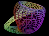
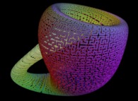
with {u,v} on the preceding curve C to fill the surface with C....
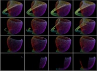
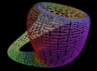
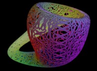
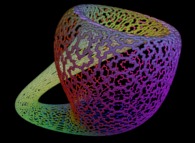
Here are some examples of this process
:
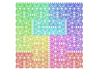
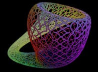
| Surface | ==> | C Curve | ==> | Surface filling Curve |
 | ==> |  | ==> |  |
 | ==> |  | ==> |  |
 | ==> |  | ==> |  |
 | ==> |  | ==> |  |
 | ==> |  | ==> |  |
 | ==> |  | ==> |  |
 | ==> |  | ==> |  |
 | ==> |  | ==> |  |
 | ==> |  | ==> |  |
4-Tridimensional Manifolds:
Many tridimensional manifolds in a tridimensional space
can be defined using a set of three equations:
X = Fx(u,v,w)
Y = Fy(u,v,w)
Z = Fz(u,v,w)
with:
u ∈ [Umin,Umax]
v ∈ [Vmin,Vmax]
w ∈ [Wmin,Wmax]
[Umin,Umax]*[Vmin,Vmax]*[Wmin,Wmax] then defined a tridimensional rectangular domain D.
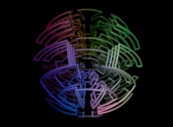
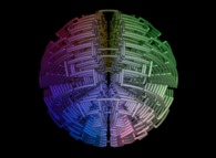
It is obvious to generalize the preceding bidimensional process in the tridimensional space...
Here are some examples of this process
:
| Tridimensional Manifold | ==> | C Curve | ==> | Tridimensional Manifold filling Curve |
5-Beyond:
Instead of using space-filling curves in order to fill the {u,v} and {u,v,w} bi- and tridimensional domains,
obviously one can use any means available and, for example, the bi-
and the tridimensional brownian motions respectively....
Here are some examples of these extended processes
:


Copyright © Jean-François COLONNA, 2023-2025.
Copyright © CMAP (Centre de Mathématiques APpliquées) UMR CNRS 7641 / École polytechnique, Institut Polytechnique de Paris, 2023-2025.

 that will be reduced
and transformed by repeating the process an infinite number of times.
To illustrate this process, here is a specific generating curve
  and the four transformations
  it must undergo at each iteration.


 ,
and again, a specific generating curve
  allows us to understand
the eight transformations
  it undergoes at each iteration.


