Visualizing with Spheres
CMAP (Centre de Mathématiques APpliquées) UMR CNRS 7641, École polytechnique, Institut Polytechnique de Paris, CNRS, France
france telecom, France Telecom R&D
[Site Map, Help and Search [Plan du Site, Aide et Recherche]]
[The Y2K Bug [Le bug de l'an 2000]]
[Real Numbers don't exist in Computers and Floating Point Computations aren't safe. [Les Nombres Réels n'existent pas dans les Ordinateurs et les Calculs Flottants ne sont pas sûrs.]]
[Please, visit A Virtual Machine for Exploring Space-Time and Beyond, the place where you can find more than 10.000 pictures and animations between Art and Science]
(CMAP28 WWW site: this page was created on 11/1/1996 and last updated on 10/03/2024 17:10:38 -CEST-)
Abstract: Computer plays today a key-role in
Science. Picture synthesis is the only way to analyse the
huge volume of results produced by Numerical Simulations.
Unfortunately the objects displayed are far from those we
experience in our everyday life. Choosing arbitrary shapes
or again colors can lead us to erroneous analysis. In this
short note we promote the use of one of the simplest
geometric object as an almost universal neutral viualization
medium.
Keywords: Scientific visualization, Numerical Simulation,
Virtual Experimentation, Sphere.
Today, computers are omnipresent in our
laboratories; in this short note I should like to
focus on the so-called Numerical Simulation.
Mathematics is the language used to write natural
laws; equations studied by mathematicians and
physicians are so complex that they cannot be
solved without the help of computers. Speeds of
more than one hundred mega-flops are common
today and some of the fastest computers are close
to reach the tera-flops level. Then we are able to
produce huge amount of numerical results that,
thanks to computers graphics, can be analysed in
order to allow us a better understanding of the
underlying laws.
I call this process (using together numerical
simulation and picture synthesis), Virtual Experimentation
[01]. Scientists are then faced with
two major dangers (traps?):
- neclegting effects of rounding-off errors
as already described in [02][03],
- using Picture Synthesis as a neutral tool.
This last point can be illustrated with what
can be said to be the simplest case of Scientific
Visualization: the one of a bidimensional scalar
field. As a matter of fact, it is the simplest case
because the display medium is bidimensional too
(for example, a computer screen); then a trivial
mapping exists between the numerical values and
the picture and each {x,y} value can be
visualized as a colored pixel. But an important
question has to be answered: how to assign
colors to each numerical value? To show there is
unfortunately no unique answer,
this picture  uses four color palettes to visualize the
same bidimensional scalar field; it displays
four very different pictures; for example:
- with or without periodical structures,
- with or without discontinuities.
The conclusion we can draw from this is
straightforward: in the field of scientific
visualization, things must be kept as simple and as
neutral as possible... I should like to extend this
point of view with problems of a higher
complexity.
Even if bidimensional
scalar fields are of a great interest (see for example
the so-called bidimensional fluid dynamics), our
computers allow us today the study of much more
complex spaces: bidimensional manifolds
embedded in tridimensional spaces, tridimensional
vector fields,...
One of the simplest geometrical
object, the sphere, can be there very useful and
the use of spheres is already quite natural  in a lot of problems.
A sphere can be defined with the following
attributes:
- the coordinates {Xc,Yc,Zc} of its center C,
- its radius r,
- its color given as a {R,G,B} vector (∈ [0,1]x[0,1]x[0,1])
-the alpha-channel will be ignored here in order to keep things simple-.
Moreover, the sphere is one of the easiest
graphical object to visualize...
Let's start with scalar mono- and bidimensional data.
For the sphere paradigm to be helpful, we
must sample these data; I call this process atomization.
This process will give us a set of
points; each of them will be visualized as a
lighted sphere centered on it (by the way, these
sets can be very far from our daily experiments;
then, tridimensional clues must be given -like
depth cueing or again fog effects, see [04]-). Its
radius r and its {R,G,B} color are available to
display a maximum of four different scalar values
Vi where i ∈ [1,4] (for the sake of simplicity, it is
assumed that Vi are non negative; if not, it
suffices to apply appropriate linear
transformations); this will help correlating
different data sets.
The four parameters r and {R,G,B} can be
defined as follows:
                    r = f (V )
                         r  i


                    R = f (V )
                         R  i


                    V = f (V )
                         V  i


                    B = f (V )
                         B  i
but it is strongly suggested to keep things as
simple as possible in order to avoid
misconstructions. Here are some straightforward
advices:
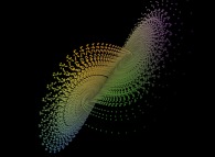
As examples,the Lorenz attractor  is displayed using
one sphere for each time step, when
the atomization process for the Jeener surface 1
  reveals the intricate inside details without the ambiguities of transparencies,
when the apparent variation of sphere sizes (due to the projection) gives a good
depth information.
All that have been said previously can be extended to
scalar tridimensional data:
spheres can be used to display voxels [05][06]
As a matter of fact, the
atomization process allows us to see through
things without the ambiguities of transparencies
(without forgetting the limits of this last process
when there are to much levels of transparent sets).
All that was said previously remains true; but in
this case the ability to move around the scene, to
penetrate inside it, is more than important. Then,
when displaying time-dependent data, it is
necessary to be careful because two time
parameters have to be displayed simulteneously:
- the data time Td (for example, the t variable used in a numerical simulation),
- the observator time To (the one that controls the change of viewing parameters).
Except for entertainment purposes, it is
suggested to freeze To during Td evolutions and
inversely. One more time, things must be kept
simple for a better understanding (let's recall there
picture synthesis is used in this context as a
scientific tool!).
A tridimensional fractal field  is a good example of this process.
All preceding advices were given for scalar data sets.
In fact, spheres can be used to display non scalar data and
for example vector fields. As a matter of fact,
instead of using only one sphere for each data
point, it is possible to use two or more aligned
spheres to display a vector  ; their attributes (ie. r
and {R,G,B}) can be kept constant or not in order
to exhibit gradient-like properties. It is
straigthforward all this can be extended to much
more complex structures.
Today, the discovery of rules for a fair use of
Scientific Visualization must be a priority for
everyone involved (software designers, engineers
and scientists). Many decades ago it has been
done for geographical maps, road signs,... and it
works! In the scientific context, on the one hand
we must never forget that there is no neutral tool
and on the other hand we must define codes that
will help to be bound toward what I shall call the
Scientific Visualization Objectivity.
- [01]
Please, visit the "Virtual Experimentation (A Virtual Space-Time Travel)" WWW site.
- [02]
"The subjectivity of computers",
Jean-François COLONNA, Technical Correspondence,
Communications of the ACM, volume 36, numero
8, page 15-18, 08/1993.
- [03]
"Kepler, Von Neumann and God (More rounding-off error visualizations)",
Jean-François COLONNA, The Visual Computer (1996), 12:346-349.
- [04]
"Creativity and Simplicity",
Jean-François COLONNA, The visual Computer (1994),10:239-242.
- [05]
"Computer Graphics, Principles and
Practice", page 549, James D. Foley, Andries van
Dam, Steven K. Feiner, John F. Hughes,
Addison-Wesley Publishing Company, 1990.
- [06]
"Volume Visualization", Arie Kaufman,
IEEE Computer Society Press Tutorial, 1990.
Copyright © Jean-François COLONNA, 1996-2024.
Copyright © France Telecom R&D and CMAP (Centre de Mathématiques APpliquées) UMR CNRS 7641 / École polytechnique, Institut Polytechnique de Paris, 1996-2024.

 uses four color palettes to visualize the
same bidimensional scalar field; it displays
four very different pictures; for example:
 in a lot of problems.

 is displayed using
one sphere for each time step, when
the atomization process for the Jeener surface 1
  reveals the intricate inside details without the ambiguities of transparencies,
when the apparent variation of sphere sizes (due to the projection) gives a good
depth information.
 is a good example of this process.
 ; their attributes (ie. r
and {R,G,B}) can be kept constant or not in order
to exhibit gradient-like properties. It is
straigthforward all this can be extended to much
more complex structures.