• 1.1-The recursive subdivision algorithm
• 1.2-The superposition of independent two-dimensional meshes

• 2.1-Definitions
• 2.2-The hyperfield
• 2.3-The N-dimensional fractal field

• 3.1-Earthquakes
• 3.2-Cloud dynamics

1.1-The recursive subdivision algorithm:

To generate, for example, mountain surfaces using fractal techniques, they are well known methods like Fourier transform of white noise and recursive subdivision [01][02]. The first one is slow, and the second one shows artifacts. Let's recall it. This algorithm starts with a triangle or a quadrilateral: for this last case, let {V(1),V(2),V(3),V(4)} be the initial two-dimensional quadrilateral; on each side {V(i),V(i+1)} let's choose (deterministically or randomly) a point P(i,i+1) and inside of {V(1),V(2),V(3),V(4)} a fifth point P. Then the five points P, P(1,2), P(2,3), P(3,4) and P(4,1) are randomly moved along the third dimension, thus giving birth to four new "three-dimensional" quadrilaterals:


• {V(1),P(1,2),P,P(4,1),V(1)},
• {P(1,2),V(2),P(2,3),P,P(1,2)},
• {P(2,3),V(3),P(3,4),P,P(2,3)},
• {P(3,4),V(4),P(4,1),P,P(3,4)}.

Then the process is iterated recursively for each new quadrilateral; at the end, we obtain an irregular surface. This process frequently shows artefacts (like creases of slope discontinuities [02]) and cannot model easily smooth terrains.





1.2-The superposition of independent two-dimensional meshes:

We propose a new method based on the superposition of independent N-dimensional meshes. To be clear, let's describe it with a two-dimensional example. We shall use a set of square meshes {M(1),M(2),...,M(m)} of decreasing sizes (the smallest one is on the order of the pixel size). We never require coincidences between nodes belonging to various meshes, unlike the recursive subdivision algorithm; thus the computations of all the meshes will be independent. For the mesh M(k) (k ∈ [1,m]) we generate on each vertex V(i,j) a random value RDN(i,j,k,S) as a function of i and j (the coordinates relating to the mesh M(k)), k (the rank of the mesh) and S (a seed for the random generator). Then the mesh is "rasterized" in the following way: if the current point P(x,y) is a vertex V(i,j), it will receive the value RDN(i,j,k,S), otherwise, its value will be interpolated between the values of its neighbours. 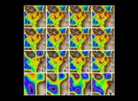Finally, a two-dimensional field is obtained by superposing and adding point by point all the rasterized meshes; figures , and show the sixteen first steps of this iterative process. Then this field can be visualized as a two-dimensional field, as a three-dimensional surface (the value at the point P(x,y) giving the third coordinate), or again transformed (see figure ) and combined with other two-dimensional fields (see figures and ). The appendix gives a view of the available tools for the manipulation of two-dimensional fields.

With this two-dimensional example, it may be seen that this method gives us four "degrees of freedom":


• the geometry of the meshes,
• the interpolation function,
• the random generator,
• and finally the mapping function between meshes and space coordinates.

Two interpolation functions have been implemented: bi-linear and bi-cubic. When used with meshes such that:

                                  size(M(k-1))
                    size(M(k)) = --------------
                                       2

and such that one vertex of M(k) coincide with one vertex of M(k-1), the bi-linear interpolation can simulate the subdivision algorithm; but unfortunately, this method (the fastest) shows clearly slope discontinuities, when the bi-cubic one looks more realistic.

2.1-Definitions:

Let E be a subset of R^n with coordinates {x(1),x(2),...,x(n)}. Let {M(1),M(2),...,M(k),...,M(m)} be a family of hypercellular meshes of decreasing sizes:

                    size(M(1)) > size(M(2)) >...> size(M(k)) >...> size(M(m)).

It is important to notice that this family is not obtained with a recursive subdivision and that all its elements are independent. Let RDN(x(1),x(2),...,x(n),k,S) be a random generator; its arguments are the coordinates {x(1),x(2),...,x(n)}, the rank k of the current mesh M(k) and a seed S.





2.2-The hyperfield:

For each point (x(1),x(2),...,x(n)) of E and for each mesh M(k) we define a scalar hyperfield Fk:

                    Fk(x(1),x(2),...,x(n),k,S) = RDN(x(1),x(2),...,x(n),k,S)

if the point {x(1),x(2),...,x(n)} of E is a vertex of the current mesh M(k), and:

                    Fk(x(1),x(2),...,x(n),k,S) = Interpolation(RDN(X(1),X(2),...,X(n),k,S))

computed for all adjoining vertices {X(1),X(2),...,X(n)} otherwise.

Here again, the Interpolation function is an arbitrary one: it can be a n-linear one using the 2^n nearest nodes, a n-cubic one, or again, any other function. This is just another parameter...





2.3-The N-dimensional fractal field:

For each point }x(1),x(2),...,x(n)} of E we define a N-dimensional fractal field F:

                                               k=m
                                              -----
                                              \
                    F(x(1),x(2),...,x(n),S) = /     p(k).Fk(x(1),x(2),...,x(n),k,S)
                                              -----
                                               k=1

where p(k) is a ponderation factor such that:

                    p(1) > p(2) >...> p(k) >...>  p(m).

The way p(k) is defined is arbitrary, but can be chosen, for example, proportional to the volume of the elementary cell of the mesh M(k).

3.1-Earthquakes:

It suffice to use the preceding model with the following mapping between S (= R^3) and E:

                    x -->  x(1),
                    y -->  x(2),
                    t -->  x(3).

Figure shows sixteen frames from a terrific (because of the amplitude...) earthquake simulation. Each of the "instaneous" mountains is obtained with a two-dimensional cross-section inside the three-dimensional fractal field at t=x(3)=constant; then this "sub-field" is visualized as a three-dimensional surface.





3.2-Cloud dynamics:

It suffice to use the preceding model with the following mapping between S (= R^3 to reduce the computing time) and E:

                    x --> [x(1) + dx(1,x(3))]
                                             modulo L
                                                     x


                    y --> [x(2) + dx(2,x(3))]
                                             modulo L
                                                     y


                    t --> [x(3)]
                                modulo L
                                        t

where the vector {dx(1,x(3)),dx(2,x(3))} is used to simulate the effect of the wind in the (x,y) plane, and the modulo operators are here to allow the generation of periodic sequences. Figure shows us a complex scene: a fractal mountain obtained by the preceding method of superposition, with three two-dimensional fields of clouds with a wind blowing from the right to the left:

                    dx(1,x(3)) = -PositiveValue.x(3),
                    dx(2,x(3)) = 0.

This simulation was only three-dimensional in order to reduce the computing time. About the shadows, the ones relating to the mountains are correct, when the ones relating to the clouds are simulated (due to their two-dimensionality...) with a texture mapping approach: at time t, a texture using the clouds at time t+Dt (Dt << Lt) is computed and then mapped onto the mountain surface.

                    display(mountain(fractal_nD(parameters),parameters),parameters);

                    fractal_nD parameters | mountain parameters | display parameters