Hilbert Curves and Infinite Knots
CMAP (Centre de Mathématiques APpliquées) UMR CNRS 7641, École polytechnique, Institut Polytechnique de Paris, CNRS, France
[Site Map, Help and Search [Plan du Site, Aide et Recherche]]
[The Y2K Bug [Le bug de l'an 2000]]
[Real Numbers don't exist in Computers and Floating Point Computations aren't safe. [Les Nombres Réels n'existent pas dans les Ordinateurs et les Calculs Flottants ne sont pas sûrs.]]
[Please, visit A Virtual Machine for Exploring Space-Time and Beyond, the place where you can find more than 10.000 pictures and animations between Art and Science]
(CMAP28 WWW site: this page was created on 05/16/2022 and last updated on 01/16/2025 11:27:16 -CET-)
[en français/in french]
In the year 1890 Giuseppe Peano discovered curves that are going through all the points of a square (and of a cube) showing then
continuous surjections between [0,1] and [0,1]x[0,1] (and [0,1]x[0,1]x[0,1]).
During the following years, David Hilbert defined more such curves that can be generalized.
The bidimensional Hilbert Curves:
Let's C1(T) being
a parametric curve  defined by means of 2 real functions of T
(T ∈ [0,1])
X1(T) ∈ [0,1] and Y1(T) ∈ [0,1]
such as
:
X1(T=0)=0 Y1(T=0)=0 (lower left corner)
X1(T=1)=1 Y1(T=1)=0 (lower right corner)
Then one defines a sequence of curves Ci(T) (i >= 1) as follows
:
Ci(T) = {Xi(T),Yi(T)} ∈ [0,1]x[0,1] --> Ci+1(T) = {Xi+1(T),Yi+1(T)} ∈ [0,1]x[0,1]
                    if T ∈ [0,1/4[:
                              Xi+1(T) =   Yi(4T-0)
                              Yi+1(T) =   Xi(4T-0)
                                                   Transformation 1
                    if T ∈ [1/4,2/4[:
                              Xi+1(T) =   Xi(4T-1)
                              Yi+1(T) = 1+Yi(4T-1)
                                                   Transformation 2
                    if T ∈ [2/4,3/4[:
                              Xi+1(T) = 1+Xi(4T-2)
                              Yi+1(T) = 1+Yi(4T-2)
                                                   Transformation 3
                    if T ∈ [3/4,1]:
                              Xi+1(T) = 2-Yi(4T-3)
                              Yi+1(T) = 1-Xi(4T-3)
                                                   Transformation 4
Please note that 4=2d where d=2 is the space dimension.
See a special C1(T) curve  in order to understand the geometrical meaning of the 4 transformations
  and of their order
  .
.
Here are the five first bidimensional Hilbert curves with an increasing number of iterations
:


 [See the used color set to display the parameter T]
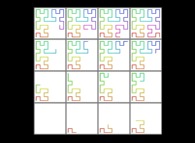
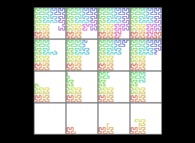
See the construction of some of them
:



Here are some examples of Hilbert-like bidimensional curves using different generating curves
:


Here is the "mapping" of a few pictures by means of a bidimensional Hilbert curve:
:
 | ==>
[iteration 11] | 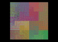 |
 | ==>
[iteration 10] | 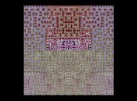 |
 | ==>
[iteration 9] | 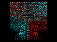 |
 | ==>
[iteration 10] | 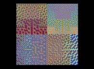 |
The tridimensional Hilbert Curves:
Let's C1(T) being
a parametric curve  defined by means of 3 real functions of T
(T ∈ [0,1])
X1(T) ∈ [0,1], Y1(T) ∈ [0,1] and Z1(T) ∈ [0,1]
such as
:
X1(T=0)=0 Y1(T=0)=0 Z1(T=0)=0 (lower left foreground corner)
X1(T=1)=1 Y1(T=1)=0 Z1(T=1)=0 (lower right foreground corner)
Then one defines a sequence of curves Ci(T) (i >= 1) as follows
:
Ci(T) = {Xi(T),Yi(T),Zi(T)} ∈ [0,1]x[0,1]x[0,1] --> Ci+1(T) = {Xi+1(T),Yi+1(T),Zi+1(T)} ∈ [0,1]x[0,1]x[0,1]
                    if T ∈ [0,1/8[:
                              Xi+1(T) =   Xi(8T-0)
                              Yi+1(T) =   Zi(8T-0)
                              Zi+1(T) =   Yi(8T-0)
                                                   Transformation 1
                    if T ∈ [1/8,2/8[:
                              Xi+1(T) =   Zi(8T-1)
                              Yi+1(T) = 1+Yi(8T-1)
                              Zi+1(T) =   Xi(8T-1)
                                                   Transformation 2
                    if T ∈ [2/8,3/8[:
                              Xi+1(T) = 1+Xi(8T-2)
                              Yi+1(T) = 1+Yi(8T-2)
                              Zi+1(T) =   Zi(8T-2)
                                                   Transformation 3
                    if T ∈ [3/8,4/8[:
                              Xi+1(T) = 1+Zi(8T-3)
                              Yi+1(T) = 1-Xi(8T-3)
                              Zi+1(T) = 1-Yi(8T-3)
                                                   Transformation 4
                    if T ∈ [4/8,5/8[:
                              Xi+1(T) = 2-Zi(8T-4)
                              Yi+1(T) = 1-Xi(8T-4)
                              Zi+1(T) = 1+Yi(8T-4)
                                                   Transformation 5
                    if T ∈ [5/8,6/8[:
                              Xi+1(T) = 1+Xi(8T-5)
                              Yi+1(T) = 1+Yi(8T-5)
                              Zi+1(T) = 1+Zi(8T-5)
                                                   Transformation 6
                    if T ∈ [6/8,7/8[:
                              Xi+1(T) = 1-Zi(8T-6)
                              Yi+1(T) = 1+Yi(8T-6)
                              Zi+1(T) = 2-Xi(8T-6)
                                                   Transformation 7
                    if T ∈ [7/8,1]:
                              Xi+1(T) =   Xi(8T-7)
                              Yi+1(T) = 1-Zi(8T-7)
                              Zi+1(T) = 2-Yi(8T-7)
                                                   Transformation 8
Please note that 8=2d where d=3 is the space dimension.
See a special C1(T) curve  in order to understand the geometrical meaning of the 8 transformations
  and of their order
  .
.
Here are the four first tridimensional Hilbert curves with an increasing number of iterations
:


 [See the used color set to display the parameter T]
See the construction of one of them
:


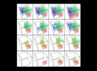

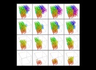
Here are some examples of Hilbert-like tridimensional curves using different generating curves and in
particular "open" knots
:




[More information about Peano Curves and Infinite Knots -in english/en anglais-]
[Plus d'informations à propos des Courbes de Peano et des Nœuds Infinis -en français/in french-]
The infinite knots:
Nota:
A mathematical node is a closed curve but to be used as a C1(T)-like curve it has to be open
(for the sake of readability, the two "free" extremities of the Ci(T) curves are not linked:
they are the lower foreground cube vertices, at left and at right respectively displayed as bigger spheres...).
Let's use a 3-foil torus knot  as the parametric curve C1(T) and let's open it
  .
.
Here are the five first curves
Ci(T) (i ∈ [1,5]):


 See the used color set to display the parameter T.
After an infinite number of iterations the curve fills the [0,1]x[0,1]x[0,1] cube: it is a first "infinite knot"...
Now, let's use a 5-foil torus knot  as the parametric curve C1(T) and let's open it
  .
.
Here are the five first curves
Ci(T) (i ∈ [1,5])
giving after an infinite number of iterations a second "infinite knot"
:


 See the used color set to display the parameter T.
Now, let's use a 7-foil torus knot  as the parametric curve C1(T) and let's open it
  .
.
Here are the five first curves
Ci(T) (i ∈ [1,5])
giving after an infinite number of iterations a third "infinite knot"
:


 See the used color set to display the parameter T.
At last, it is obviously possible to fill
more "complex" tridimensional manifolds than a cube and for example:
| Tridimensional Manifold | ==> | C Curve | ==> | Tridimensional Manifold filling Node |
Copyright © Jean-François COLONNA, 2022-2025.
Copyright © CMAP (Centre de Mathématiques APpliquées) UMR CNRS 7641 / École polytechnique, Institut Polytechnique de Paris, 2022-2025.

 defined by means of 2 real functions of T
(T ∈ [0,1])
X1(T) ∈ [0,1] and Y1(T) ∈ [0,1]
such as
:
 in order to understand the geometrical meaning of the 4 transformations
  and of their order
  .
.


 [See the used color set to display the parameter T]


 defined by means of 3 real functions of T
(T ∈ [0,1])
X1(T) ∈ [0,1], Y1(T) ∈ [0,1] and Z1(T) ∈ [0,1]
such as
:
 in order to understand the geometrical meaning of the 8 transformations
  and of their order
  .
.


 [See the used color set to display the parameter T]


 as the parametric curve C1(T) and let's open it
  See the used color set to display the parameter T.
 as the parametric curve C1(T) and let's open it
  See the used color set to display the parameter T.
 as the parametric curve C1(T) and let's open it
  See the used color set to display the parameter T.

